Treatment of experimental errors and estimation of uncertainties

The experimental errors are divided into two classes: those which are due to the limited statistic of the measurement and those which are due to systematic effect, like for example wrong energy calibration. Modern DIS experiments have very small statistical uncertainties so that the contribution of systematic uncertainties becomes dominant. Many systematics are correlated between the various data points used in the fit. Almost all up-to-date analyses include a full treatment of all correlated experimental errors. Two main methods have been used to propagate uncertainties on the fitted data points to the PDF uncertainties: the Hessian method which is based on linear error propagation through the covariance error matrix and the Monte-Carlo sampling method which has been used in conjunction with neural networks. In both methods the global accuracy of the fit is defined as a χ 2 summed on all data sets. In fits not including correlated errors, one would minimize a simple χ 2 function defined as

χ 2= Σ expt Σ Nei =1(Di − Ti)2/ σ 2i

where Ne is the number of cross section data points in experiment e,Di is a data value, Ti is the corresponding theoretical value of the cross section calculated from the parameterisedparton distributions function and σ i is the experimental errors. Ideally we would expect the errors to be given by the choice of tolerance Δχ 2=1 for the 68 % (one-sigma) confidence level limit and Δχ 2=2.71 for the 90 % (two-sigma) confidence level limit, which are the well grounded statistical expectations. This is appropriate when fitting consistent data sets with well-defined theory like in HERAPDF analysis where only DIS data from HERA experiments have been used. In global fits from CTEQ and MSTW analyses which include DIS and hadron-hadron data, the fitting procedure tends to provide an unrealistically small uncertainty. There are discrepancies much larger than the error band between the fitted cross section and individual experiments. This is likely due to some failure of the theoretical and model approximation to work properly over the whole range of the data and may be due to some sources of experimental data errors not being properly quantified. Instead a much weaker “hypothesis-testing” criterion has been appealed. The tolerance Δχ 2 is determined from the criterion that each individual data set should be described within its 68 (or 90) % limit. In MSTW, one of the most commonly used PDF extraction, the tolerances are tuned for each data set. They are in the region Δχ 2 ≤ 50 for a 90 % confidence limit. In CTEQ, the other most commonly used global analysis, the 90 % confidence limit errors correspond to the choice Δχ 2=100 which is an average over all data sets. Recently, the NNPDF global analysis based on an input distribution parameterised with a neural-network as a set of very flexible parton distribution functions with about 200 parameters and using the same input data as CTEQ and NNPDF, has obtained an error band with very good consistency of all data sets with statistical expectations. This may indicate that the large tolerances in the CTEQ and MSTW analyses is partly due to the lack of flexibility of the parameterisations and that the large tolerances do not only reflect the experimental errors of the input data but also some model and theory uncertainties.

Model uncertainties

The model uncertainties are related to the assumptions made in PDF extraction. There is not a unique way to estimate the model uncertainties. They may contribute implicitly to the large tolerances as defined by CTEQ and MSTW. Often the groups prefer to illustrate the model uncertainties as a variant of PDF sets rather than including them as errors added to the experimental errors. A few examples of uncertainties are due to:

• Input distributions

The usual choice of the parametric form of the input distributions is arbitrary. Varying the analytic form of the input distribution can be quite sizeable and even dominant over all other errors (see Aaron et al., 2010). The error is estimated by comparing various parameterisations which give a good description the DIS data and have the smallest number of parameters. It is however difficult to fully quantify this uncertainty as far as the analytic shape of the parton distributions is not known. The GJR group has used a dynamical model to limit the uncertainty from this source. In the model the evolution of the input distributions starts at very low Q2(Q20 ≈ 0.4GeV2) where the nucleon only consists of valence quarks. Sea quarks and gluons are generated through the DGLAP equations. It provides a much narrower uncertainty at small x but this seems a very low scale to use DGLAP equations. All other groups have preferred not to use this additional physical assumption. The opposite approach is the very flexible parameterisation of the neural network (NNPDF) analysis. It has some ambiguity from the procedure to determine the central values and uncertainties and it provides larger errors but it is free of debatable physical assumptions.

• Flavour symmetry

There is no reason to assume that at low x the sea is flavour symmetric. It has been commonly assumed that s=s¯=(u¯+d¯)/4 at the input scale Q20. The suppression factor of the strange sea is due to its larger mass. More sophisticated assumptions, not assuming that the strange sea has the same shape as the up and down quarks at high x, have also been used (CTEQ and MSTW). DIS and Drell-Yan experiments have shown that the density of anti-quarks u¯ and d¯ quarks are not equal at x above 0.01. There is however not a unique description of the difference u¯ − d ¯. NNPDF has a very flexible parametrisation of the strange sea at small x.

• Heavy quark treatment

It is usually assumed that all heavy quarks (charm, beauty and top) are radiatively generated from the gluon and light quarks by QCD evolution to large Q2 starting from a null distribution below an energy threshold at approximately the relevant quark mass. It has become clear in recent years that the treatment of the heavy quark (charm and beauty) threshold is a delicate issue. Several heavy quarks treatments (commonly called schemes) have been considered. In all schemes the choice of the heavy quark masses is arbitrary. So far, the scheme dependence is not systematically taken into account in the fits. See for example the detailed discussion in MSTW08 (Martin et al. 2008). It has little impact on the valence quark distributions, but affects directly the gluon and heavy quark distributions.

• Coupling constant α s (Q2)

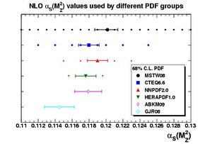
Figure 3: A compilation of the values of α s (M2Z0) and its uncertainties used by the most recent PDFs analyses (MSTWPDF [1]).

A fundamental uncertainty is the value of the QCD coupling constant, α s (Q2). The PDF fits are sensitive to the value of α s and can be used as a mean of determining its value. Much more information on the value of α s than present in the data sets used in the PDF fits exists, for example from the precision measurements at LEP (Bethke 2009). Some of the groups have chosen to use a fixed value in the fit, a kind of world average value, but have not yet agreed on a common value and on its uncertainty. Other groups prefer to consider α s as an additional free parameter of the fit. The value of α s has a strong impact on the gluon distribution. A figure of the values of α s (M2Z0), at the energy scale of the Z0 mass and its uncertainty, used in the most up to date fits is shown in Figure 3.

Theory uncertainties

The genuine theory uncertainties are due to the terms used to write the cross sections and to the truncation of the DGLAP perturbative expansion to formulate the evolution equations and the perturbativeexpansion of the coefficient functions. Theory uncertainties are commonly not included in the published uncertainties because they are difficult to quantify a priori until a better calculation or prescription is available. Although NLO QCD fits give a good description of the data down to Q2 values in the range 1 − 3GeV2, such fits neglect higher-order QCD terms in power of α s, including enhanced log(1/x) or log(1 − x) terms and other higher twist corrections. Rigorous calculations to NNLO are now available in DIS but they are usually used as a variant, since they have not been fully worked out for all non-DIS processes.

Results

Since about four decades ago a lot of effort has been put in measuring DIS processes and then in extracting PDFs from the data. This effort is still ongoing. It is remarkable that there is a broad agreement of all PDFs and uncertainties despite many differences in input data, methods of analysis and model assumptions. There are however discrepancies in predictions of the PDF groups which can be locally bigger than the uncertainty of each. A working group to understand the commonalities and differences between the predictions and uncertainties of the PDF groups has been set up at CERN (see PDF4LHC [4]). A benchmarking exercise was carried out to evaluate important cross sections including well established processes as W, Z and top cross sections which will be measured in the coming months at the LHC. This exercise was very instructive. For example let consider two production processes at 7 TeV energy in the centre of mass of proton-proton collision:

• Z production is mainly sensitive to the quark and antiquark densities in the proton. The impact from the variation of the value of α s is relatively small (Figure 4). The overall spread of the central value of the predictions is about nine percent and is reduced to an impressive four percent if we only consider the most global fits (CTEQ, MSTW, NNPDF).
• Production of a tt¯ pair is mainly sensitive to the gluon density. It is also very sensitive the value of α s (Figure 5). The overall spread of the central values is about eighteen percent and is of eight percent for the three most global fits. Clearly the agreement could be even better if the cross sections were evaluated at a common value of α s.

Figure 4: Cross section predictions at 7TeV for Z production (MSTWPDF [2]).

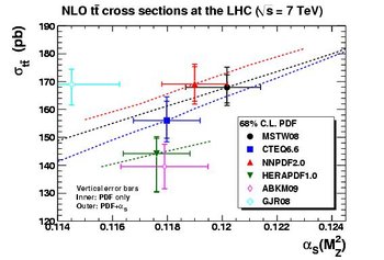
Figure 5: Cross section predictions at 7TeV for tt¯ production (MSTWPDF [3]).

Applications and prospects

In the near future new data from the Tevatron and final data from HERA, along with model and theoretical development, will allow for more precise determinations of PDFs and a better understanding of their uncertainties. Further standardizations are planned for future updates. The main application of the new parton distribution functions is at present to make predictions for physical cross sections at the proton-proton collider LHC, such as the Higgs boson production or the search for new physics in jets production at large transverse momentum. Conversely, measurements from the LHC should improve knowledge of parton distributions in a large part of the x range. Further contributions could be brought by the Relativistic Heavy Ion Collider RHIC at Brookhaven. In a few years DIS measurements at JLAB 12 GeV should bring new important constraints at large x value. More future DIS machines like LHeC at CERN and EIC in the US are being studied.

References

• F.D. Aaron et al.,[H1 and ZEUS Collaborations], JHEP 01 (2010) 109, [arXiv:0911.0884[hep-ph]].
• S. Alekhin, J. Blümlein, S. Klein and S. Moch, Phys. Rev. D81, 014032 (2010), [arXiv:0908.2766[hep-ph]].
• G. Altarelli and G. Parisi, Nucl. Phys. B126, 298 (1977).
• D. Ball et al., [The NNPDF Collaboration],[arXiv:1002.4407[hep-ph]].
• S. Bethke, Eur. Phys. J. C64, 689 (2009), [arXiv:0908.1135[hep-ph]].
• J.C. Collins, D.E. Soper and G. Sterman,[arXiv:0409.313[hep-ph]].
• A. DeRujula et al., Phys. Rev. D10, 1649 (1974).
• Yu. L. Dokshitzer, Sov. Phys. JETP 46, 641 (1977).
• M. Glück, P. Jimenez-Delgado and E. Reya, Eur. Phys. J. C53, 355 (2008), [arXiv:0709.0614[hep-ph]].
• V.N. Gribov and L.N. Lipatov, Sov. J. Nucl. Phys. 15, 438 (1972).
• A.D. Martin, W.J. Stirling, R.S. Thorne and G.Watt, Eur. Phys. J. C63, 189 (2009), [arXiv:0901.0002[hep-ph]].
• P.M. Nadolsky et al., Phys. Rev. D78, 013004 (2008), [arXiv:0802.0007[hep-ph]].
• J. Pumplin et al., JHEP 0207 (2002) 012, [arXiv:0201195v3 [hep-ph].

http://www.scholarpedia.org/article/Introduction_to_Parton_Distribution_Functions