
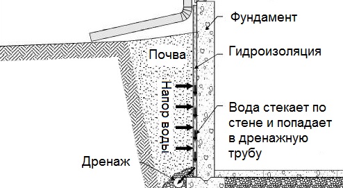
Общие условия выбора системы дренажа: Система дренажа выбирается в зависимости от характера защищаемого...
Археология об основании Рима: Новые раскопки проясняют и такой острый дискуссионный вопрос, как дата самого возникновения Рима...
Общие условия выбора системы дренажа: Система дренажа выбирается в зависимости от характера защищаемого...
Археология об основании Рима: Новые раскопки проясняют и такой острый дискуссионный вопрос, как дата самого возникновения Рима...
Топ:
Установка замедленного коксования: Чем выше температура и ниже давление, тем место разрыва углеродной цепи всё больше смещается к её концу и значительно возрастает...
Основы обеспечения единства измерений: Обеспечение единства измерений - деятельность метрологических служб, направленная на достижение...
Интересное:
Что нужно делать при лейкемии: Прежде всего, необходимо выяснить, не страдаете ли вы каким-либо душевным недугом...
Средства для ингаляционного наркоза: Наркоз наступает в результате вдыхания (ингаляции) средств, которое осуществляют или с помощью маски...
Отражение на счетах бухгалтерского учета процесса приобретения: Процесс заготовления представляет систему экономических событий, включающих приобретение организацией у поставщиков сырья...
Дисциплины:
|
из
5.00
|
Заказать работу |
|
|
|
|
IntroductiontoPartonDistributionFunctions
| JoëlFeltesse (2010), Scholarpedia, 5(11):10160. | doi:10.4249/scholarpedia.10160 | revision #186761 [ link to/cite this article ] |
Post-publication activity
Curator: JoëlFeltesse
The momentum distribution functions of the partons within the proton are called Parton Distribution Functions.
Contents
[hide]
|
Definition of PDFs
The Parton name was proposed by Richard Feynman in 1969 as a generic description for any particle constituent within the proton, neutron and other hadrons. These particles are referred today as quarks and gluons.
There are six types of quarks, known as flavours: up (u), down (d), charm (c), strange (s), top (t) and bottom (b). The antiparticles of quarks are antiquarks. Quarks have various intrinsic properties, including electric charge, spin, mass and colour charge.
Quarks carry a fractional electric charge of value, either -1/3 or +2/3 times the elementary charge (where the electron has -1 unit), depending on flavour. Up, charm and top quarks have a charge +2/3, while down, strange and bottom quarks have -1/3. The quarks which determine the quantum numbers of hadrons are called constituent or valence quarks. For example the proton is composed of two up quarks (referred below as uv quark) and one down quark (referred below as dv quark), and the neutron of two down quarks and one up quark.
Quarks are spin 1/2 particles. The spin direction is called polarisation.
Quarks possess a property called colour charge. There are three types of colour charge. Each quark carries a colour. The system of attraction and repulsion between coloured quarks is called strong interaction, which is mediated by force carrying particles known as gluons. Gluons, like the photons are massless, have a spin of 1 and no electric charge but carry colour charge. The theory that describes strong interactions is called Quantum Chromodynamics (QCD).
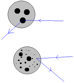
The three-quark model assuming that a proton or a neutron is made of three free non-interacting quarks in a bag is too simple. It cannot match a scattering process like the inelastic scattering of electrons off protons. Those valence quarks are imbedded in a sea of virtual quark-antiquark pairs generated by the gluons which hold the quarks together in the proton. All of these particles - valence quarks, sea quarks and gluons- are partons.
The partonic structure of a nucleon is best probed in scattering processes like Deep Inelastic Scattering (DIS) of leptons (electrons, muons or neutrinos) off nucleons, where the lepton acts as a probe which transfers a four momentum of modulus q to the nucleon in the collision. The Nobel Prize was awarded to Jerome Friedman, Henry Kendall and Richard Taylor in 1990 for their pioneering electron-proton DIS experiment at SLAC in 1966 which first provided evidence for a partonic structure of the nucleon.
|
|
In DIS the resolving power of the probe is approximately ℏ /q and so the level of structure revealed increases with q. For q=100GeV, the resolution is roughly 0.002fm, sufficient to probe the internal structure of the nucleon. It is convenient to consider a frame in which the target nucleon has a very large momentum. In such a frame the momentum of the parton is almost collinear with the nucleon momentum, so that the target can be seen as a stream of partons, each carrying a fraction x of the longitudinal momentum. The momentum distribution functions of the partons within the proton are simply called Parton Distribution Functions (PDFs) when the spin direction of the partons is not considered. They represent the probability densities (strictly speaking they rather represent number densities as they are normalised to the number of partons) to find a parton carrying a momentum fraction x at a squared energy scale Q2 (= − q 2). DIS experiments have shown that the number of partons goes up at low x with Q2, and falls at high x. At low Q2 the three valence quarks become more and more dominant in the nucleon. At high Q2 there are more and more quark-antiquark pairs which carry a low momentum fraction x. They constitute the sea quarks. A salient finding of the DIS experiments is that the quarks and antiquarks only carry about half of the nucleon momentum, the remainder being carried by the gluons. The fraction carried by gluons increases with increasing Q2.
The central feature of QCD is the asymptotic freedom discovered in 1973 by David Gross, David Politzer and Frank Wilczek (Nobel Prize in 2004). It implies that interactions between partons within a nucleon becomes arbitrarily weak at shorter distances. QCD gives quantitative predictions about the rate of change of parton distributions when the Q2 energy scale varies. It is governed by the QCD evolution equations for parton densities from (Gribov and Lipatov 1972), (Altarelli and Parisi 1977) and (Dokshitzer 1977) (DGLAP) in the domain where perturbative calculations can be applied, that is in the limit where the running coupling constant of α s (Q2) of QCD is much smaller than one (α s (Q2) ≪ 1). The equations have been formulated at different level of approximations, relative to different power of α s (Q2) in the perturbative development, usually named as Leading-Order (LO), i.e. first order in α s (Q2), Next-to-Leading-Order (NLO) and Next-to-Next–Leading-Order (NNLO). In the following we will consider Parton Distributions Functions obtained with evolution equations at the most widely used order.
The DGLAP differential equations give the Q2 dependence but cannot make a definitive prediction of the x dependence of the parton distributions at a given Q2. It has to be extracted from the data. The parton distributions are related to the observable cross sections by the QCD factorisation theorems (see for example (Collins, Soper and Sterman 2009)). The cross section of a hard process can be written as a calculable parton interaction convoluted with the parton densities. The factorisation theorems are the whole basis to extract the PDFs from some processes and to apply perturbative calculations to many important processes involving hadrons. In DIS it reads
|
|
σ (x,Q2) ≈ Σ aCa ⊗ fa /A(x,Q2)+remainder
Here Ca is the calculable part and fa/A is the parton distribution of parton a in a hadron of type A. The sum is over all type of partons, a. It is conventional to call the first term on the right of the above equation the leading twist contribution. The remainder is called the higher twist correction. It is formally of order 1/Q2 but not precisely known. The correction is often neglected in extracting PDFs from the cross sections. The convolution of the Ca coefficient functions with the parton distributions is not uniquely defined at NLO. Usually the Ca coefficient functions and the parton distributions are written in the Modified Minimal Subtraction Scheme of factorisation called MS-bar (see MS-bar definition of parton distribution functions).
Method of determinations
PDFs sets are obtained by a fit on a large number of cross section data points in a large grid of Q2 and x values from many experiments. The most commonly used procedure consists of parameterising the dependence of the parton distributions (quarks, antiquarks, gluon) on the variable x at some low value of Q2=Q20, which is large enough that the unknown terms of the perturbative equations are assumed to be negligible, and evolving these input distributions up in Q2 through the DGLAP equations. The number of unknown parameters is typically between 10 and 30. The factorisation theorems allow to derive predictions for the cross sections.. These predictions are then fitted to as much of the experimental data together as possible, to determine the parameters and to provide parton distributions.
Examples of PDFs
An overview of parton distributions in the proton is shown in the figures below at two scales Q=2GeV (Figure 1) and Q=100GeV (Figure 2).

Figure 1: Overview of the CTEQ6M parton distribution at Q = 2 GeV (Pumplin et al. 2002).
Figure 2: Overview of the CTEQ6M parton distribution at Q = 100 GeV (Pumplin et al. 2002).
As naively expected, at small Q2 and large x values above 0.1, the u quarks are the dominant distributions, more than twice as large as the d quarks at high x and much larger than the heavy quarks. At low x value the sea is not flavour symmetric. There are significantly less strange quarks than up and down quarks. The charm density is null below the charm threshold (mc=Q ≈ 1.5GeV) and increases slowly as energy increases. At higher Q2 (Figure 2) the shape of the quark and gluon distributions changes quickly at very low x. The sea becomes more flavour symmetric, since at low x the evolution is flavour-independent, and there are more and more sea quarks and gluons. The rise of the parton densities at low x and high Q2 values is a foundational prediction of QCD (DeRujula et al., 1974) which was clearly verified at the HERA electron-proton collider at DESY in 1993.
There is however not a unique set of Parton Distribution Functions commonly accepted. There are several groups in competition to provide the best parametrisation of parton distributions. The groups do not use the same input data. They differ mainly in the way the PDFs are parameterised, in the treatment of heavy quarks and in the value of the coupling constant α s as well in the way the experimental errors are treated and the theoretical errors are estimated.
Data sets in fit
The very extensive and precise DIS data from fixed-target lepton-nucleon scattering experiments at SLAC, FNAL, CERN and from the electron-proton HERA collider at DESY provide the backbone of parton distribution analysis. The lepton-nucleon data include electron, muon and neutrino DIS measurements on hydrogen, deuterium and nuclear targets. DIS data however are insufficient to determine accurately flavour decomposition of the quark and antiquark sea or the gluon distribution at large x. In inclusive DIS, the gluon is only probed via the rate of evolution. The additional physical processes which are used in the fits are:
|
|
The determination of the most global fits like CTEQ6.6 (Nadolsky et al. 2008), MSTW08 (Martin et al. 2008), GJR08 (Glück et al. 2008) and more recently NNPDF2.0 (Ball et al. 2010) are based on data from DIS and proton-nucleon fixed target experiments as well as results from the HERA and Tevatron colliders. The four groups do not fit exactly the same data sets, e.g. GJR has no W and Z production data. ABKM09 (Alekhin et al. 2009) fit combines DIS and fixed target Drell-Yan data. HERAPDF1.0 (Aaron et al. 2010) fit uses only HERA data.
Model uncertainties
The model uncertainties are related to the assumptions made in PDF extraction. There is not a unique way to estimate the model uncertainties. They may contribute implicitly to the large tolerances as defined by CTEQ and MSTW. Often the groups prefer to illustrate the model uncertainties as a variant of PDF sets rather than including them as errors added to the experimental errors. A few examples of uncertainties are due to:
The usual choice of the parametric form of the input distributions is arbitrary. Varying the analytic form of the input distribution can be quite sizeable and even dominant over all other errors (see Aaron et al., 2010). The error is estimated by comparing various parameterisations which give a good description the DIS data and have the smallest number of parameters. It is however difficult to fully quantify this uncertainty as far as the analytic shape of the parton distributions is not known. The GJR group has used a dynamical model to limit the uncertainty from this source. In the model the evolution of the input distributions starts at very low Q2(Q20 ≈ 0.4GeV2) where the nucleon only consists of valence quarks. Sea quarks and gluons are generated through the DGLAP equations. It provides a much narrower uncertainty at small x but this seems a very low scale to use DGLAP equations. All other groups have preferred not to use this additional physical assumption. The opposite approach is the very flexible parameterisation of the neural network (NNPDF) analysis. It has some ambiguity from the procedure to determine the central values and uncertainties and it provides larger errors but it is free of debatable physical assumptions.
There is no reason to assume that at low x the sea is flavour symmetric. It has been commonly assumed that s=s¯=(u¯+d¯)/4 at the input scale Q20. The suppression factor of the strange sea is due to its larger mass. More sophisticated assumptions, not assuming that the strange sea has the same shape as the up and down quarks at high x, have also been used (CTEQ and MSTW). DIS and Drell-Yan experiments have shown that the density of anti-quarks u¯ and d¯ quarks are not equal at x above 0.01. There is however not a unique description of the difference u¯ − d ¯. NNPDF has a very flexible parametrisation of the strange sea at small x.
It is usually assumed that all heavy quarks (charm, beauty and top) are radiatively generated from the gluon and light quarks by QCD evolution to large Q2 starting from a null distribution below an energy threshold at approximately the relevant quark mass. It has become clear in recent years that the treatment of the heavy quark (charm and beauty) threshold is a delicate issue. Several heavy quarks treatments (commonly called schemes) have been considered. In all schemes the choice of the heavy quark masses is arbitrary. So far, the scheme dependence is not systematically taken into account in the fits. See for example the detailed discussion in MSTW08 (Martin et al. 2008). It has little impact on the valence quark distributions, but affects directly the gluon and heavy quark distributions.
|
|
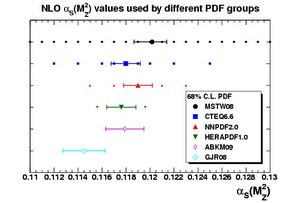
Figure 3: A compilation of the values of α s (M2Z0) and its uncertainties used by the most recent PDFs analyses (MSTWPDF [1]).
A fundamental uncertainty is the value of the QCD coupling constant, α s (Q2). The PDF fits are sensitive to the value of α s and can be used as a mean of determining its value. Much more information on the value of α s than present in the data sets used in the PDF fits exists, for example from the precision measurements at LEP (Bethke 2009). Some of the groups have chosen to use a fixed value in the fit, a kind of world average value, but have not yet agreed on a common value and on its uncertainty. Other groups prefer to consider α s as an additional free parameter of the fit. The value of α s has a strong impact on the gluon distribution. A figure of the values of α s (M2Z0), at the energy scale of the Z0 mass and its uncertainty, used in the most up to date fits is shown in Figure 3.
Theory uncertainties
The genuine theory uncertainties are due to the terms used to write the cross sections and to the truncation of the DGLAP perturbative expansion to formulate the evolution equations and the perturbativeexpansion of the coefficient functions. Theory uncertainties are commonly not included in the published uncertainties because they are difficult to quantify a priori until a better calculation or prescription is available. Although NLO QCD fits give a good description of the data down to Q2 values in the range 1 − 3GeV2, such fits neglect higher-order QCD terms in power of α s, including enhanced log(1/x) or log(1 − x) terms and other higher twist corrections. Rigorous calculations to NNLO are now available in DIS but they are usually used as a variant, since they have not been fully worked out for all non-DIS processes.
Results
Since about four decades ago a lot of effort has been put in measuring DIS processes and then in extracting PDFs from the data. This effort is still ongoing. It is remarkable that there is a broad agreement of all PDFs and uncertainties despite many differences in input data, methods of analysis and model assumptions. There are however discrepancies in predictions of the PDF groups which can be locally bigger than the uncertainty of each. A working group to understand the commonalities and differences between the predictions and uncertainties of the PDF groups has been set up at CERN (see PDF4LHC [4]). A benchmarking exercise was carried out to evaluate important cross sections including well established processes as W, Z and top cross sections which will be measured in the coming months at the LHC. This exercise was very instructive. For example let consider two production processes at 7 TeV energy in the centre of mass of proton-proton collision:

Figure 4: Cross section predictions at 7TeV for Z production (MSTWPDF [2]).
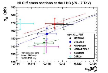
Figure 5: Cross section predictions at 7TeV for tt¯ production (MSTWPDF [3]).
Applications and prospects
In the near future new data from the Tevatron and final data from HERA, along with model and theoretical development, will allow for more precise determinations of PDFs and a better understanding of their uncertainties. Further standardizations are planned for future updates. The main application of the new parton distribution functions is at present to make predictions for physical cross sections at the proton-proton collider LHC, such as the Higgs boson production or the search for new physics in jets production at large transverse momentum. Conversely, measurements from the LHC should improve knowledge of parton distributions in a large part of the x range. Further contributions could be brought by the Relativistic Heavy Ion Collider RHIC at Brookhaven. In a few years DIS measurements at JLAB 12 GeV should bring new important constraints at large x value. More future DIS machines like LHeC at CERN and EIC in the US are being studied.
|
|
References
http://www.scholarpedia.org/article/Introduction_to_Parton_Distribution_Functions
В физике элементарных частиц модельПартона -это модель адронов, таких как протоны и нейтроны, предложенная Ричардом Фейнманом. Он полезен для интерпретации каскадов излучения (партонного ливня), образующихся в результате процессов и взаимодействий КХД при столкновениях частиц высоких энергий.
Содержание
Модель[ править ]
См. также: DGLAP
Адрон определяется в системе отсчета, где он имеет бесконечный импульс—допустимое приближение при высоких энергиях. Таким образом, движение партона замедляется замедлением времени, а распределение заряда адрона сжимается по Лоренцу, поэтому входящие частицы будут рассеиваться "мгновенно и бессвязно".]
Партоны определяются относительно физического масштаба (как исследуется обратная передача импульса).] Например, кварковыйпартон в одном масштабе длины может оказаться суперпозицией кварковогопартонного состояния с кварковымпартоном и глюоннымпартонным состоянием вместе с другими состояниями с большим количеством партонов в меньшем масштабе длины. Аналогично, глюонныйпартон в одном масштабе может распадаться на суперпозицию глюонногопартонного состояния, глюонногопартона и кварк-антикварковогопартонного состояния и других многопартонных состояний. Из-за этого число партонов в адроне фактически увеличивается с передачей импульса. ] При низких энергиях (т. е. больших масштабах длины) барион содержит три валентных партона (кварки), а мезон-два валентных партона (кварк и антикварк-партон). Однако при более высоких энергиях наблюдения показывают морские партоны (невалентныепартоны) в дополнение к валентным партонам. [8]
История[edit]
Модель Партона была предложена Ричардом Фейнманом в 1969 году и первоначально использовалась для анализа высокоэнергетических столкновений. [2] Он был применен к глубокому неупругому рассеянию электронов / протонов Бьоркеном и Пашосом.Позже, с экспериментальным наблюдением масштабирования Бьоркена, проверкой кварковоймоделии подтверждением асимптотической свободы в квантовой хромодинамике, партоны были сопоставлены с кварками и глюонами. Модель Партона остается оправданным приближением при высоких энергиях, и другие расширили теорию на протяжении многих лет[ как? ].
Это было признано[ когда? ] что партоны описывают одни и те же объекты, которые теперь чаще называют кварками и глюонами. Более подробное изложение свойств и физических теорий, косвенно относящихся к партонам, можно найти в разделе кварки.
Функции распределения Партона[ править ]
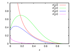
Функции распределения партонов CTEQ6 в схеме перенормировки MS и Q = 2 ГэВ для глюонов (красный), вверх (зеленый), вниз (синий) и странных (фиолетовый) кварков. На графике изображено произведение продольной доли импульса x и функций распределения f по отношению к x.
Функция распределения партона (PDF) в рамках так называемой коллинеарной факторизации определяется как плотность вероятности нахождения частицы с определенной долей продольного импульса x в масштабе разрешения Q2. Из-за присущей непертурбативной природы партонов, которые не могут наблюдаться как свободные частицы, плотности партонов не могут быть вычислены с помощью пертурбативной КХД. Однако в рамках КХД можно изучать изменение плотности партона со шкалой разрешения, обеспечиваемой внешним зондом. Такой масштаб обеспечивается например виртуальным фотоном с виртуальностью Q2 или струей Масштаб может быть вычислен по энергии и импульсу виртуального фотона или струи; чем больше импульс и энергия, тем меньше масштаб разрешения—это следствие принципа неопределенности Гейзенберга. Было обнаружено, что изменение плотности партона со шкалой разрешения хорошо согласуется с экспериментом; [9] это важный тест КХД.
Функции распределения Партона получаются путем подгонки наблюдаемых к экспериментальным данным; они не могут быть вычислены с помощью пертурбативной КХД. Недавно было обнаружено, что они могут быть вычислены непосредственно в решеточной КХД с использованием теории эффективного поля с большим импульсом [10] [11]
Экспериментально определенные функции распределения партона доступны из различных групп по всему миру. Основными неполяризованными наборами данных являются:
Библиотека LHAPDF [12] предоставляет унифицированный и простой в использовании интерфейс Fortran / C++ для всех основных наборов PDF-файлов.
Обобщенные партонные распределения (GPDS) - это более поздний подход к лучшему пониманию структуры адрона, представляющий партонные распределения как функции большего числа переменных, таких как поперечный импульс и спин партона. [13] Они могут быть использованы для изучения спиновой структуры протона, в частности, правило суммы Джи связывает интеграл GPDs с угловым моментом, переносимым кварками и глюонами. [14] Ранние названия включали "не-прямые", "не-диагональные" или "перекошенные" распределения партона. Доступ к ним осуществляется через новый класс исключительных процессов, для которых все частицы обнаруживаются в конечном состоянии, таких как глубоко виртуальное комптоновское рассеяние. [15] Обычные функции распределения партона восстанавливаются путем установки на ноль (прямой предел) дополнительных переменных в обобщенных распределениях партона. Другие правила показывают, что электрический форм-фактор, магнитный форм - фактор, или даже форм-факторы, связанные с тензором энергии-импульса, также включены в GPDS. Полное 3-мерное изображение партонов внутри адронов также может быть получено из GPDS [16]
Моделирование[ править ]
Моделирование партоновских ливней используется в вычислительной физике частиц либо для автоматического расчета взаимодействия частиц, распада или генераторов событий, и особенно важно в феноменологии БАК, где они обычно исследуются с помощью моделирования Монте-Карло. Масштаб, в котором партоны отдаются адронизации, фиксируется программой Монте-Карло Ливня. Распространенные варианты душа Монте-Карло-это ПИФИЯ и ХЕРВИГ. [17] [18]
См. также[ править ]
Ссылки[ править ]
1. ^ Дэвисон Э. Сопер, Физика партоновских ливней. Дата обращения: 17 ноября 2013 года.
2. ^ Перейти к:a b Фейнман, Р. П. (1969). "Поведение адронных столкновений при экстремальных энергиях". Столкновения высоких энергий: Третья Международная конференция в Стоуни-Брук, Нью-Йорк. Gordon&Breach. pp. 237-249. ISBN 978-0-677-13950-0.
3. ^ Перейтик:a b Bjorken, J.; Paschos, E. (1969). "Неупругое электрон-протонное и γ - протонноерассеяниеиструктурануклона ". Физический обзор. 185 (5): 1975-1982. Bibcode: 1969PhRv..185.1975 B. doi: 10.1103/PhysRev.185.1975.
IntroductiontoPartonDistributionFunctions
| JoëlFeltesse (2010), Scholarpedia, 5(11):10160. | doi:10.4249/scholarpedia.10160 | revision #186761 [ link to/cite this article ] |
Post-publication activity
Curator: JoëlFeltesse
|
|
|
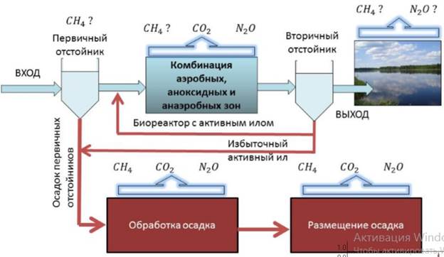
Эмиссия газов от очистных сооружений канализации: В последние годы внимание мирового сообщества сосредоточено на экологических проблемах...
Поперечные профили набережных и береговой полосы: На городских территориях берегоукрепление проектируют с учетом технических и экономических требований, но особое значение придают эстетическим...
Археология об основании Рима: Новые раскопки проясняют и такой острый дискуссионный вопрос, как дата самого возникновения Рима...
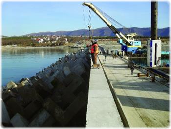
Типы оградительных сооружений в морском порту: По расположению оградительных сооружений в плане различают волноломы, обе оконечности...
© cyberpedia.su 2017-2024 - Не является автором материалов. Исключительное право сохранено за автором текста.
Если вы не хотите, чтобы данный материал был у нас на сайте, перейдите по ссылке: Нарушение авторских прав. Мы поможем в написании вашей работы!