
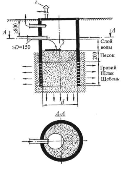
Индивидуальные очистные сооружения: К классу индивидуальных очистных сооружений относят сооружения, пропускная способность которых...
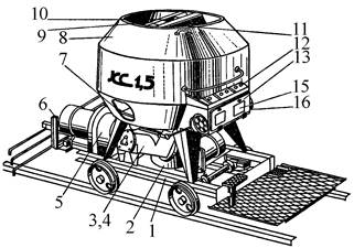
Кормораздатчик мобильный электрифицированный: схема и процесс работы устройства...
Индивидуальные очистные сооружения: К классу индивидуальных очистных сооружений относят сооружения, пропускная способность которых...
Кормораздатчик мобильный электрифицированный: схема и процесс работы устройства...
Топ:
Особенности труда и отдыха в условиях низких температур: К работам при низких температурах на открытом воздухе и в не отапливаемых помещениях допускаются лица не моложе 18 лет, прошедшие...
Оценка эффективности инструментов коммуникационной политики: Внешние коммуникации - обмен информацией между организацией и её внешней средой...
Теоретическая значимость работы: Описание теоретической значимости (ценности) результатов исследования должно присутствовать во введении...
Интересное:
Лечение прогрессирующих форм рака: Одним из наиболее важных достижений экспериментальной химиотерапии опухолей, начатой в 60-х и реализованной в 70-х годах, является...
Как мы говорим и как мы слушаем: общение можно сравнить с огромным зонтиком, под которым скрыто все...
Национальное богатство страны и его составляющие: для оценки элементов национального богатства используются...
Дисциплины:
|
из
5.00
|
Заказать работу |
Содержание книги
Поиск на нашем сайте
|
|
|
|
Now let's look at a function to compute enough terms in the Fibonacci sequence so the ratio is less than the correct machine epsilon (eps) for datatype single or double. % How many terms needed to get single precision results?
fibodemo('single')
% How many terms needed to get double precision results?
fibodemo('double')
% Now let's look at the working code.
type fibodemo
% Notice that we initialize several of our variables, |fcurrent|,
% |fnext|, and |goldenMean|, with values that are dependent on the
% input datatype, and the tolerance |tol| depends on that type as
% well. Single precision requires that we calculate fewer terms than
% the equivalent double precision calculation.
ans = 19
ans = 41
function nterms = fibodemo(dtype)
%FIBODEMO Used by SINGLEMATH demo.
% Calculate number of terms in Fibonacci sequence.
fcurrent = ones(dtype);
fnext = fcurrent;
goldenMean = (ones(dtype)+sqrt(5))/2;
tol = eps(goldenMean);
nterms = 2;
while abs(fnext/fcurrent - goldenMean) >= tol
nterms = nterms + 1;
temp = fnext;
fnext = fnext + fcurrent;
fcurrent = temp;
end
Inverses of Matrices
This demo shows how to visualize matrices as images and uses this to illustrate matrix inversion.
This is a graphic representation of a random matrix. The RAND command creates the matrix, and the IMAGESC command plots an image of the matrix, automatically scaling the color map appropriately.
n = 100;
a = rand(n);
imagesc(a);
colormap(hot);
axis square;

This is a representation of the inverse of that matrix. While the numbers in the previous matrix were completely random, the elements in this matrix are anything BUT random. In fact, each element in this matrix ("b") depends on every one of the ten thousand elements in the previous matrix ("a").
b = inv(a);
imagesc(b);
axis square;

But how do we know for sure if this is really the correct inverse for the original matrix? Multiply the two together and see if the result is correct, because just as 3*(1/3) = 1, so must a*inv(a) = I, the identity matrix. The identity matrix (almost always designated by I) is like an enormous number one. It is completely made up of zeros, except for ones running along the main diagonal.
This is the product of the matrix with its inverse: sure enough, it has the distinctive look of the identity matrix, with a band of ones streaming down the main diagonal, surrounded by a sea of zeros.
imagesc(a*b);
axis square;

Graphs and Matrices
This demo gives an explanation of the relationship between graphs and matrices and a good application of SPARSE matrices.
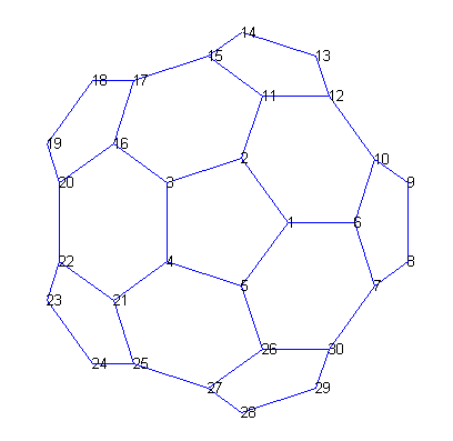
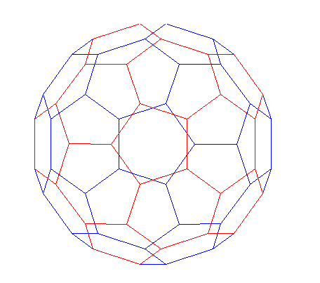
A graph is a set of nodes with specified connections between them. An example is the connectivity graph of the Buckminster Fuller geodesic dome (also a soccer ball or a carbon-60 molecule).
In MATLAB, the graph of the geodesic dome can be generated with the BUCKY function.% Define the variables.
[B,V] = bucky;
H = sparse(60,60);
k = 31:60;
H(k,k) = B(k,k);
% Visualize the variables.
gplot(B-H,V,'b-');
hold on
gplot(H,V,'r-');
hold off
axis off equal

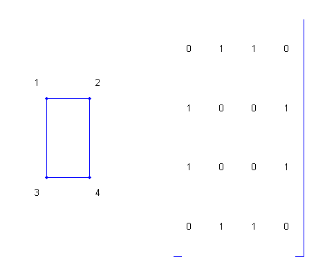
A graph can be represented by its adjacency matrix.
To construct the adjacency matrix, the nodes are numbered 1 to N. Then element (i,j) of the matrix is set to 1 if node i is connected to node j, and 0 otherwise. % Define a matrix A.
A = [0 1 1 0; 1 0 0 1; 1 0 0 1; 0 1 1 0];
% Draw a picture showing the connected nodes.
cla
subplot(1,2,1);
gplot(A,[0 1;1 1;0 0;1 0],'.-');
text([-0.2, 1.2 -0.2, 1.2],[1.2, 1.2, -.2, -.2],('1234')',...
'HorizontalAlignment','center')
axis([-1 2 -1 2],'off')
% Draw a picture showing the adjacency matrix.
subplot(1,2,2);
xtemp=repmat(1:4,1,4);
ytemp=reshape(repmat(1:4,4,1),16,1)';
text(xtemp-.5,ytemp-.5,char('0'+A(:)),'HorizontalAlignment','center');
line([.25 0 0.25 NaN 3.75 4 4 3.75],[0 0 4 4 NaN 0 0 4 4])
axis off tight
Here are the nodes in one hemisphere of the bucky ball, numbered polygon by polygon.subplot(1,1,1);
gplot(B(1:30,1:30),V(1:30,:),'b-')
for j = 1:30,
text(V(j,1),V(j,2),int2str(j),'FontSize',10);
end
axis off equal
To visualize the adjacency matrix of this hemisphere, we use the SPY function to plot the silhouette of the nonzero elements.
Note that the matrix is symmetric, since if node i is connected to node j, then node j is connected to node i.
spy(B(1:30,1:30))
title('spy(B(1:30,1:30))')

numbering of one hemisphere into the other.
[B,V] = bucky;
H = sparse(60,60);
k = 31:60;
H(k,k) = B(k,k);
gplot(B-H,V,'b-');
hold on
gplot(H,V,'r-');
for j = 31:60
text(V(j,1),V(j,2),int2str(j),...
'FontSize',10,'HorizontalAlignment','center');
end
hold off
axis off equal

Finally, here is a SPY plot of the final sparse matrix.
spy(B)
title('spy(B)')

In many useful graphs, each node is connected to only a few other nodes. As a result, the adjacency matrices contain just a few nonzero entries per row.
This demo has shown one place where SPARSE matrices come in handy.gplot(B-H,V,'b-');
axis off equal
hold on
gplot(H,V,'r-')
hold off
|
|
|
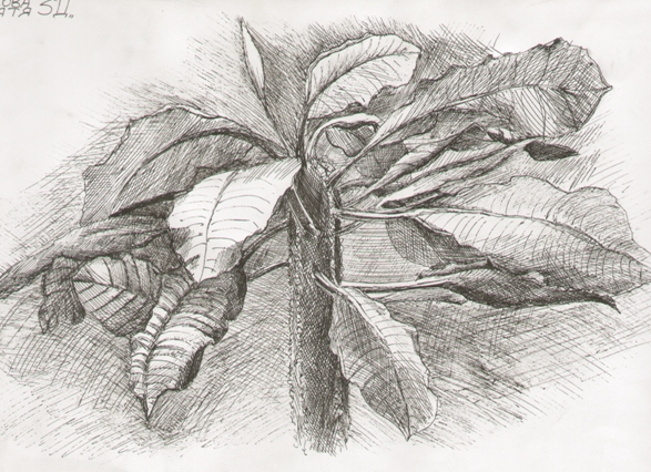
Наброски и зарисовки растений, плодов, цветов: Освоить конструктивное построение структуры дерева через зарисовки отдельных деревьев, группы деревьев...
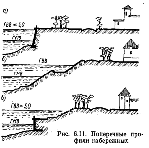
Поперечные профили набережных и береговой полосы: На городских территориях берегоукрепление проектируют с учетом технических и экономических требований, но особое значение придают эстетическим...
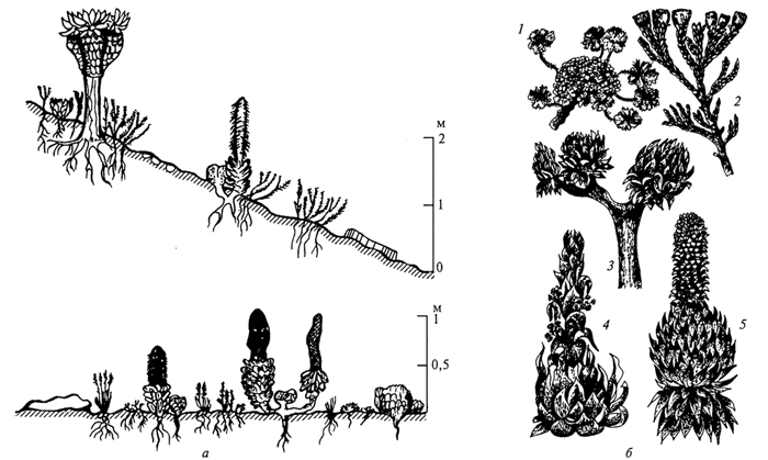
Адаптации растений и животных к жизни в горах: Большое значение для жизни организмов в горах имеют степень расчленения, крутизна и экспозиционные различия склонов...
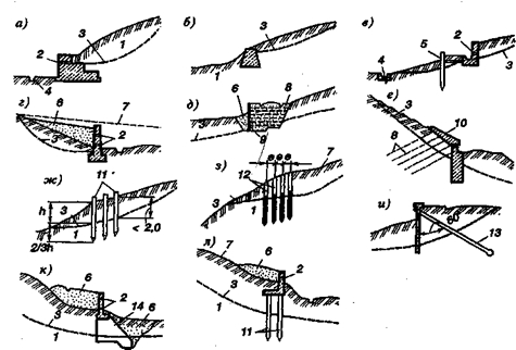
Механическое удерживание земляных масс: Механическое удерживание земляных масс на склоне обеспечивают контрфорсными сооружениями различных конструкций...
© cyberpedia.su 2017-2025 - Не является автором материалов. Исключительное право сохранено за автором текста.
Если вы не хотите, чтобы данный материал был у нас на сайте, перейдите по ссылке: Нарушение авторских прав. Мы поможем в написании вашей работы!

