
Типы оградительных сооружений в морском порту: По расположению оградительных сооружений в плане различают волноломы, обе оконечности...

Семя – орган полового размножения и расселения растений: наружи у семян имеется плотный покров – кожура...
Типы оградительных сооружений в морском порту: По расположению оградительных сооружений в плане различают волноломы, обе оконечности...
Семя – орган полового размножения и расселения растений: наружи у семян имеется плотный покров – кожура...
Топ:
Марксистская теория происхождения государства: По мнению Маркса и Энгельса, в основе развития общества, происходящих в нем изменений лежит...
Оснащения врачебно-сестринской бригады.
Характеристика АТП и сварочно-жестяницкого участка: Транспорт в настоящее время является одной из важнейших отраслей народного хозяйства...
Интересное:
Национальное богатство страны и его составляющие: для оценки элементов национального богатства используются...
Подходы к решению темы фильма: Существует три основных типа исторического фильма, имеющих между собой много общего...
Распространение рака на другие отдаленные от желудка органы: Характерных симптомов рака желудка не существует. Выраженные симптомы появляются, когда опухоль...
Дисциплины:
|
из
5.00
|
Заказать работу |
|
|
|
|
|
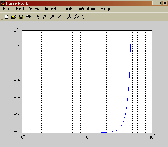
» x=logspace(-1,3);
» loglog(x.*exp(x)./x)
» grid on
semilogx(...) — строит график функции в логарифмическом масштабе (основание 10) по оси X и линейном по оси Y; semilogy (...) — строит график функции в логарифмическом масштабе по оси Y и линейном по оси X.

|
» х=0:0.5:10;
» semilogy(x.exp(x))
>> grid on
Построение гистограмм
>> x=-3:0.2:3;
>> y=randn(1000,1);
>> hist(y,x)
>> help randn
RANDN Normally distributed random numbers.
RANDN(N) is an N-by-N matrix with random entries, chosen from a normal distribution with mean zero, variance one and standard deviation one.
RANDN(M,N) and RANDN([M,N]) are M-by-N matrices with random entries. RANDN(M,N,P,...) or RANDN([M,N,P...]) generate random arrays. RANDN with no arguments is a scalar whose value changes each time it is referenced. RANDN(SIZE(A)) is the same size as A.
RANDN produces pseudo-random numbers. The sequence of numbers generated is determined by the state of the generator. Since MATLAB resets the state at start-up, the sequence of numbers generated will be the same unless the state is changed.
S = RANDN('state') is a 2-element vector containing the current state of the normal generator. RANDN('state',S) resets the state to S. RANDN('state',0) resets the generator to its initial state. RANDN('state',J), for integer J, resets the generator to its J-th state.
RANDN('state',sum(100*clock)) resets it to a different state each time.
MATLAB Version 4.x used random number generators with a single seed. RANDN('seed',0) and RANDN('seed',J) cause the MATLAB 4 generator to be used. RANDN('seed') returns the current seed of the MATLAB 4 normal generator. RANDN('state',J) and RANDN('state',S) cause the MATLAB 5 generator to be used.
See also RAND, SPRAND, SPRANDN, RANDPERM.

|
Bar plot of a bell shaped curve
x = -2.9:0.2:2.9;
bar(x,exp(-x.*x));

Stairstep plot of a sine wave
x=0:0.25:10;
stairs(x,sin(x));

Errorbar plot
x=-2:0.1:2;
y=erf(x);
e = rand(size(x))/10;
errorbar(x,y,e);

Polar plot
t=0:.01:2*pi;
polar(t,abs(sin(2*t).*cos(2*t)));

Stem plot
x = 0:0.1:4;
y = sin(x.^2).*exp(-x);
stem(x,y)

XYZ plots in MATLAB.
D Surface Plots
>> graf3d
Demonstrate Handle Graphics for surface plots in MATLAB. This window allows you to assemble a string of MATLAB commands that results in a plot in
the axis in the upper left corner.
By playing with the popup menus on the right side of the window, you can adjust the type of plot, the type of shading, the color map,
|
|
and so on.
The MiniCommand Window in the lower
right shows the list of commands that create
the plot. If you like, you can even directly edit
the commands in the MiniCommand Window.
Type control-return to execute code in the
MiniCommand Window.
Line Plotting
>> hndlgraf
Demonstrates Handle Graphics for line plots in MATLAB. This window allows you to assemble a string of MATLAB commands that results in a plot in
the axis in the upper left corner.
By playing with the popup menus on the right side of the window, you can adjust the line style of the plot, the line width, the marker size, and the color using Handle Graphics.
The MiniCommand Window in the lower right shows the list of commands that create the plot. If you like, you can even directly edit the commands in the MiniCommand Window. Type control-return to execute code in the
MiniCommand Window.
Axes Properties
>> hndlaxis
Demonstrates Handle Graphics for axes in MATLAB.
This window allows you to assemble a string
of MATLAB commands that results in a plot in
the axis in the upper left corner.
By playing with the popup menus on the right
side of the window, you can adjust the scaling
for the axes, the grid lines, the direction of the
plot and the color of the axes using Handle
Graphics.
The MiniCommand Window in the lower
right shows the list of commands that create
the plot. If you like, you can even directly edit
the commands in the MiniCommand Window.
Type control-return to execute code in the
MiniCommand Window.
P = round(poly(A)) % The characteristic polynomial of a matrix
P =
1 -5 5 -1
R = roots(P) % Roots of a polynomial
R =
3.7321
1.0000
0.2679
Q = conv(P,P) % Convolve two vectors
R = conv(P,Q)
Q = 1 -10 35 -52 35 -10 1
R = 1 -15 90 -278 480 -480 278 -90 15 -1
stem(R); % Plot the result

|
|
|
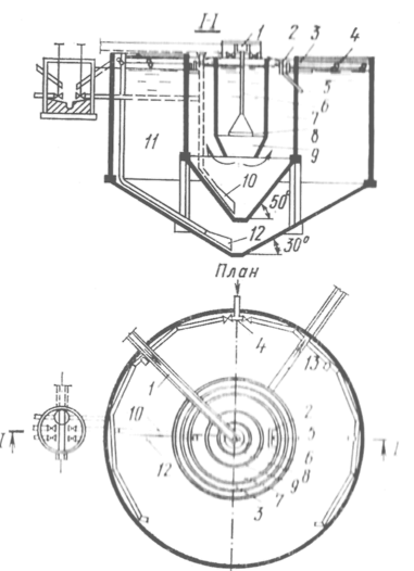
Типы сооружений для обработки осадков: Септиками называются сооружения, в которых одновременно происходят осветление сточной жидкости...
Поперечные профили набережных и береговой полосы: На городских территориях берегоукрепление проектируют с учетом технических и экономических требований, но особое значение придают эстетическим...
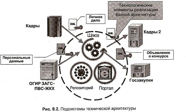
Архитектура электронного правительства: Единая архитектура – это методологический подход при создании системы управления государства, который строится...
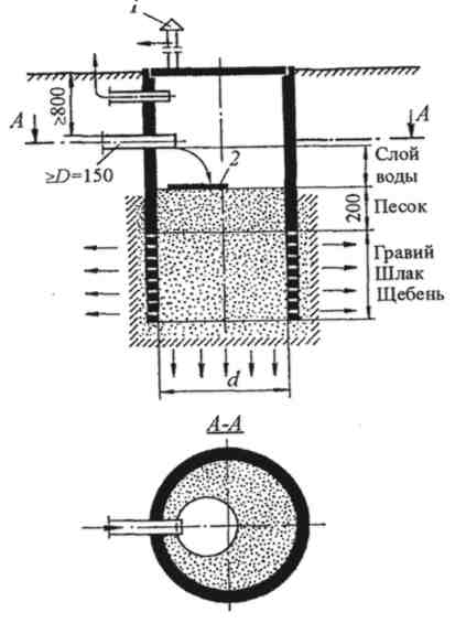
Индивидуальные очистные сооружения: К классу индивидуальных очистных сооружений относят сооружения, пропускная способность которых...
© cyberpedia.su 2017-2024 - Не является автором материалов. Исключительное право сохранено за автором текста.
Если вы не хотите, чтобы данный материал был у нас на сайте, перейдите по ссылке: Нарушение авторских прав. Мы поможем в написании вашей работы!